My Review Note for Applied Machine Learning (First Half)
Why this post
This semester I am taking Applied Machine Learning with Andreas Mueller. It’s a great class focusing on the practical side of machine learning.
As the midterm is coming, I am revising for what we have covered so far, and think that preparing a review note would be an effective way to do so (though the exam is closed book). I am posting my notes here so it can benefit more people.
Acknowledgment
The texts of this note are largely inspired by:
- Course material for COMS 4995 Applied Machine Learning.
The example codes in this note are modified based on:
- Course material for COMS 4995 Applied Machine Learning.
- Supplemental material of An Introduction to Machine Learning with Python by Andreas C. Müller and Sarah Guido (O’Reilly). Copyright 2017 Sarah Guido and Andreas Müller, 978-1-449-36941-5.
Care has been taken to avoid copyrighted contents as much as possible, and give citation wherever is proper.
Introduction to Machine Learning
Type of machine learnings
- Supervised (function approximation + generalization; regression v.s. classification)
- Unsupervised (clustering, outlier detection)
- Reinforcement Learning (explore & learn from the environment)
- Others (semi-supervised, active learning, forecasting, etc.)
Parametric and Non-parametric models
- Parametric model: Number of “parameters” (degrees of freedom) independent of data.
- e.g.: Linear Regression, Logistic Regression, Nearest Shrunken Centroid
- Non-parametric model: Degrees of freedom increase with more data. Each training instance can be viewed as a “parameter” in the model, as you use them in the prediction.
- e.g.: Random Forest, Nearest Neighbors
Classification: From binary to multi-class
- One v.s. Rest (OvR) (standard): needs n binary classifiers; predict the class with highest score.
- One v.s. One (OvO): needs \(n \cdot (n-1) / 2\) binary classifiers; predict by voting for highest positives
How to formalize a machine learning problem in general
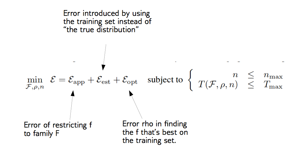
\[\min_{f \in F} \sum_{i=1}^N{L(f(x_i),y_i) + \alpha R(f)}\]We want to find the \(f\) in function family \(F\) that minimizes the error (risk, denoted by function \(L\)) on the training set, and at the same time keeps it simple (denoted by the regularized term \(R\) and \(\alpha\)).
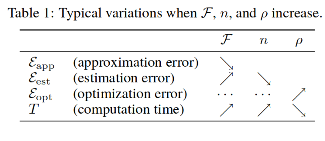
Decomposing Generalization Error (Bottou et. al, picture from Applied ML course note aml-06, page 28 & 29)
Difference between Machine Learning and Statistics
| ML | Statistics |
|---|---|
| Data First | Model First |
| Prediction + Generalization1 | Inference |
Guideline Principles in Machine Learning
- Defining the goal, and measurement (metrics) of the goal
- Thinking about the context: baseline and benefit
- Communicating the result: how explainable is the model/result?
- Ethics
- Data Collection (More data? What is the cost?)
The Machine Learning Workflow 2

Information Leakage
Data Leakage is the creation of unexpected additional information in the training data, allowing a model or machine learning algorithm to make unrealistically good predictions. Leakage is a pervasive challenge in applied machine learning, causing models to over-represent their generalization error and often rendering them useless in the real world. It can caused by human or mechanical error, and can be intentional or unintentional in both cases.
Source: https://www.kaggle.com/wiki/Leakage
Common mistakes include:
- Keep features that are not available in new data
- Leaking of information from the future into the past
- Do preprocessing on the whole dataset (before train/test split)
- Test on test data sets multiple times
Git
For git, I have found the following 2 YouTube videos very helpful:

The following slide by Andreas Mueller is also a very good one (which explains git reset, git revert, etc. which I did not cover in this note:
Below I summarized some key points about git:
- Create/Remove repository:
git init # use git to track current directory rm .git # undo the above (your files are still there) - Typical workflow:
git clone [url] # clone a remote repository git branch newBranch # create a new branch git checkout newBranch # say "Now I want to work on that branch" # do your job... git add this_file # add it to staging area git commit # Take a snapshot of the state of the folder, with a commit message. It will be identified with an ID (hash value) git push origin master # push from local -> remote git pull origin master # pull from remote -> local git merge A # merge branch A to current branch - My favorite shortcuts/commands:
git checkout -b newBranch # create branch and checkout in one line
git add -A # update the indices for all files in the entire working tree
git commit -a # stage files that have been modified and deleted, but not new files you have not done git add with
git commit -m <msg> # use the given <msg> as the commit message.
git stash # saves your local modifications away and reverts the working directory to match the HEAD commit. Can be used before a git pull
Note that
git add -Aandgit commit -amay accidentally commit things you do not intend to, so use them with caution! - Other important ones (in lecture notes or used in Homework 1):
git reset --soft <commit> # moves HEAD to <commit>, takes the current branch with it git reset --mixed <commit> # moves HEAD to <commit>, changes index to be at <commit>, but not working directory git reset --hard <commit> # moved HEAD to <commit>, changes index and working tree to <commit> git rebase -i <commit> # interactive rebase git rebase --onto feature master~3 master # rebase everything from master~2 (master - 3 commits, excluding this one) up until the tip of master (included) to the tip of feature. git reflog show # show reference logs that records when the tips of branches and other references were updated in the local repository. git checkout HEAD@{3} # checkout to the commit where HEAD used to be three moves ago git checkout feature this_file # merge the specific file (this_file) from feature to your current branch git log # show git log -
The hardest part of git in my opinion is the “polymorphism” of git commands. As shown above, you can do git checkout on a branch, a commit, a commit + a file, and they all mean different things. (This motivates me to write a git tutorial in the future when I have time, where I will go through the common git commands in a different way as existing tutorials.)
-
Difference (Relationship) between git and github: people new to git may be confused by those two. In one sentence: Git is a version control tool, and GitHub is an online project hosting platform using git.(Therefore, you may use git with or without Github.)
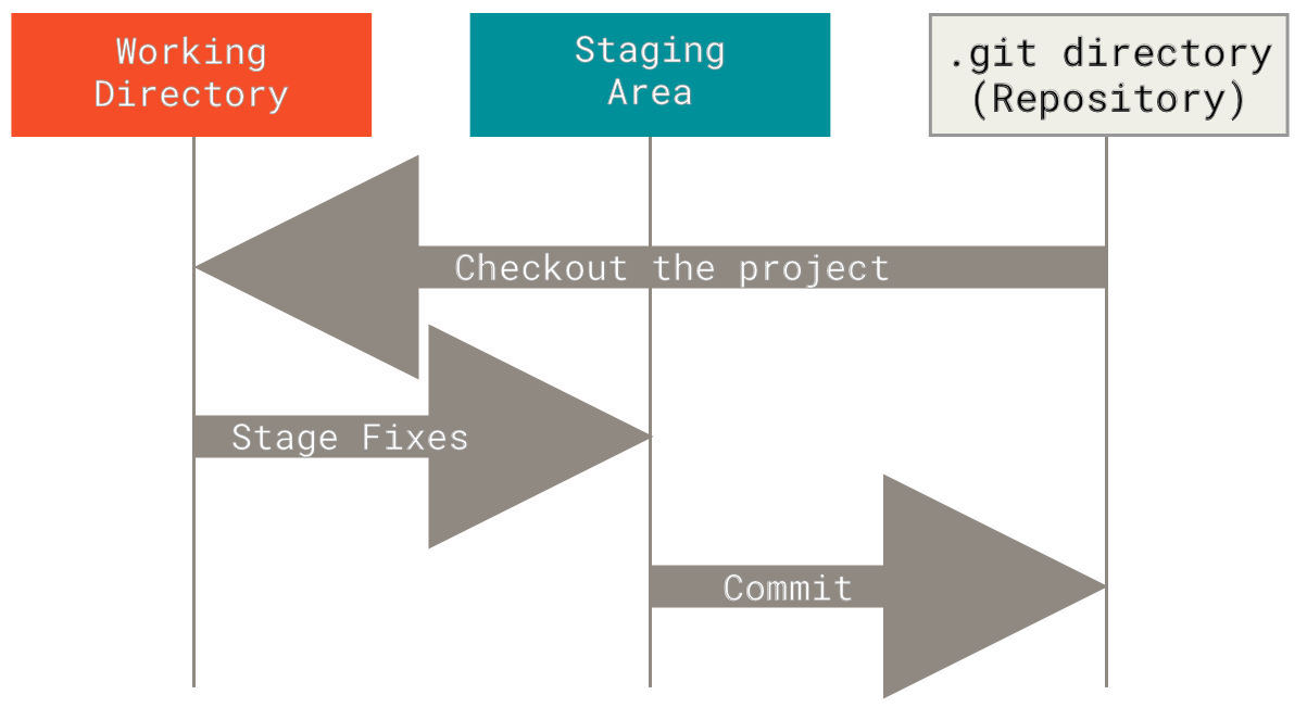
- Git add and staging area3:
- Fast-forward 4 (Note that no new commit is created):
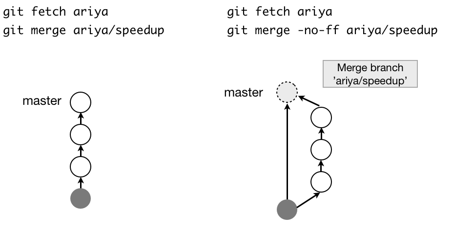
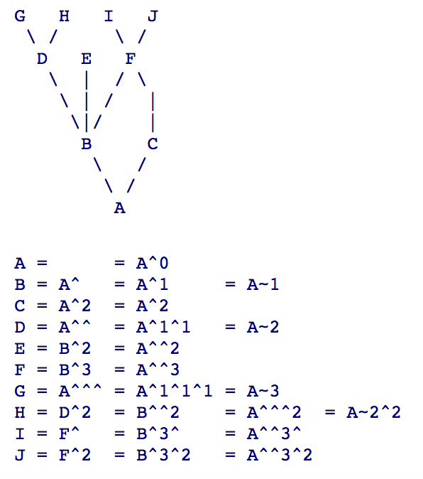
- What is HEAD^ and HEAD~ 5:
- Github Pull Request:
-
Pull requests allow you to contribute to a repository which you don’t have permission to write to. The general workflow is: fork -> clone to local -> add a feature branch -> make changes -> push.
-
To keep update with the upstream, you may also need to: add upstream as another remote -> pull from upstream -> work upon it -> push to your origin remote.
-
Coding Guidelines:
Good resources (and books that I really like):
- Pep 8
- Refactoring: Improving the Design of Existing Code by Kent Beck and Martin Fowler
- Clean Code: A Handbook of Agile Software Craftsmanship by Robert Cecil Martin
Python:
Python Quick Intro:
- Powerful
- Simple Syntax
- Interpreted language: slow (many libraries written in C/Fortran/Cython)
- Python 2 v.s. Python 3 (main changes in: division, print, iterator, string; need something from python 3 in python 2? do
from __future__ import bla) - For good practices, always use explicit imports and standard naming
conventions. (Don’t
from bla import *!)
Testing and Documentation:
Different kinds of tests
- Unit Tests: a function is doing the right thing; Can be done with pytest
- Integration tests: functions together are doing the right thing; Can be done with TravisCI (continuous integration)
- Non-regression tests: bugs truly get removed
Different ways of doing documentation:
- PEP 257 for docstrings and inline comments
- NumpyDoc format
- Various tools for generating documentation pages: SPhinx, ReadTheDocs
Visualization – Exploration and Communications
Visual Channels: Try not to…
- Use 3D-volume to show information
- Use textures to show information
- Use hues for quantitative changes
- Use bad colormaps such as jet and rainbow. They vary non-linearly and non-monotonically in lightness, which can create edges in images where there are none. The varying lightness also makes grayscale print completely useless.
Color maps:
| Sequential Colormaps | Diverging Colormaps | Qualitative Colormaps | Miscellaneous Colormaps |
|---|---|---|---|
| Go from one hue/saturation to another (Lightness also changes) | Grey/white (focus point) in the middle, different hues going in either direction | Use to show discrete values | Don’t use jet and rainbow! (Andy will be disappointed if you do so @.@) |
| Use to emphasize extremes | Use to show deviation from the neutral points | Designed to have optimum contrast for a particular number of discrete values | Use perceptual uniform colormaps |
Matplotlib Quick Intro:
% matplotlib inlinev.s.% matplotlib notebookin Jupyter Notebook- Figure and Axes:
- Create automatically by doing plot command
- Create by
plt.figure() - Create by
plt.subplots(n,m) - Create by
plt.subplot(n, m, i), where i is 1-indexed, column-based position - Two interfaces:
- Stateful interface: applies to current figure and axes (e.g.:
plt.xlim) - Object-oriented interface: explicitly use object (e.g.:
ax.set_xlim)
- Stateful interface: applies to current figure and axes (e.g.:
Important commands:
- Plot command
ax.plot(np.linspace(-4, 4, 100), sin, '--o', c = 'r', lw = 3)- Use figsize to specify how large each plot is (otherwise it will be “squeezed”)
- Single variable x: plot it against its index; Two variables x and y: plot against each other
- By default, it’s line-plot. Use “o” to create a scatterplot
- Can change the width, color, dashing and markers of the plot
- Scatter command:
ax.scatter(x, y, c=x-y, s=np.abs(np.random.normal(scale=20, size=50)), cmap='bwr', edgecolor='k')- cmap is the colormap, bwr means blue-white-red
- k is black
- Histogram:
ax.hist(np.random.normal(size=100), bins="auto")- Use bins=”auto” to heuristically choose number of bins
- Bar chart (vertical):
plt.bar(range(len(value)), value); plt.xticks(range(len(value)), labels, rotation=90)- For bar chart, the length must be provided. This can be done using range and len.
- Bar chart (horizontal):
plt.barh(range(len(value)), value); plt.yticks(range(len(value)), labels, fontsize=10) - Heatmap:
ax[0, 1].imshow(arr, interpolation='bilinear')- imshow essentially renders numpy arrays as images
- Hexgrids:
plt.hexbin(x, y, bins='log', extent=(-1, 1, -1, 1))- hexbin is essentially a 2-D histogram with hexagonal cells. (which is used to show 2D density map)
- It can be much more informative than a scatter plot
- TwinX:
ax2 = ax1.twinx()- Show series in different scale much better
Fight Against Overfitting
Naive Way: No train/test Split
Drawback
You never know how your model performs on new data, and you will cry.
First Attempt: Train Test Split (by default 75%-25%)
Code
from sklearn.model_selection import train_test_split
X_train, X_test, y_train, y_test = train_test_split(X, y)
Drawback
If we use the test error rate to tune hyper-parameters, it will learn about noise in the test set, and this knowledge will not generalize to new data.
Key idea: You should only touch your test data once.
Second Attempt: Three-fold split (add validation set)
Code
from sklearn.model_selection import train_test_split
X_trainval, X_test, y_trainval, y_test = train_test_split(X, y)
X_train, X_val, y_train, y_val = train_test_split(X_trainval, y_trainval)
Pros
Fast and simple
Cons
We lose a lot of data for evaluation, and the results depend on the particular sampling. (overfit on validation set)
Third Attempt: K-fold Cross Validation + Train/Test split
Idea
Split data into multiple folds and built multiple models. Each time test models on different (unused) fold.
Code
from sklearn.model_selection import cross_val_score
scores = cross_val_score(knn, X_trainval, y_trainval, cv=10) # equiv to StratifiedKFold without shuffle
print(np.mean(scores), np.std(scores))
Pros
- Each data point is in the test-set exactly once.
- Better data use (larger training sets)
Cons
- It takes 5 or 10 times longer (you train 5/10 models)
More CV strategies
Code
from sklearn.model_selection import KFold, ShuffleSplit, StratifiedKFold
kfold = KFold(n_splits=10)
ss = ShuffleSplit(n_splits=30, train_size=.7, test_size=.3)
skfold = StratifiedKFold(n_splits=10)
Explanation
- Stratified K-Fold: preserves the class frequencies in each fold to be the same as of the overall dataset
- Especially helpful when data is imbalanced
- Leave One Out: Equivalent to
KFold(n_folds=n_samples), where we use n-1 samples to train and 1 to test.- Cons: high variance, and it takes a long time!
- Solution: Repeated (Stratified) K-Fold + Shuffling: Reduces variance, so better!
- ShuffleSplit: Repeatedly and randomly pick training/test sets based on training/test set size for number of iterations times.
- Pros: Especially good for subsample when data set is large
- GroupKFold: Patient example; where samples in the same group are highly correlated. New data essentially means new group. So we want to split data based on group.
- TimeSeriesSplit: Stock price example; Taking increasing chunks of data from the past and making predictions on the next chunk. Making sure you do not have access to the “future”.
Final Attempt 1: Use GridSearch CV that wraps up everything
Code
from sklearn.model_selection import GridSearchCV

X_train, X_test, y_train, y_test = train_test_split(X, y, stratify=y)

param_grid = {'n_neighbors':  np.arange(1, 20, 3)}
grid = GridSearchCV(KNeighborsClassifier(), param_grid=param_grid, cv=10)
grid.fit(X_train, y_train)
print(grid.best_score_, grid.best_params_) #grid also has grid.cv_results_ which has many useful statistics
Note
- We still need to split our data into training and test set.
- If we do GridSearchCV on a pipeline, the param_grid’s key should look like:
'svc__C:'.
Final Attempt 2: Use built-in CV for specific models
Code
from sklearn.linear_model import RidgeCV
ridge = RidgeCV().fit(X_train, y_train)
print(ridge.score(X_test, y_test))
print(ridge.alpha_)
Note
- Usually those CV are more efficient.
- Support: RidgeCV(), LarsCV(), LassoLarsCV(), ElasticNetCV(), LogisticRegressionCV().
- We also have RFECV (efficient cv for recursive feature elimination) and CalibratedClassifierCV (Cross validation for calibration)
- All have reasonable built-in parameter grids.
- For RidgeCV you can’t pick the “cv”!
Preprocessing
Dealing with missing data: Imputation
In real life it’s very common that the data set is not clean. There are missing values in it. We need to fill them in before training model using it.
Imputaion methods
- Mean/median
- KNN: find k nearest neighbors that have non-missing values and average their values; tricky if there is no feature that is always non-missing. (we need such to find nearest neighbors)
- Model driven: Train regression model for missing values, can also do this iteratively. Very flexible methods
- Iterative
- fancyimpute: Has many methods; MICE (Reimplementation of Multiple Imputation by Chained Equations), more details here
Code
from sklearn.preprocessing import Imputer
imp = Imputer(strategy="mean").fit(X_train)
X_mean_imp = imp.transform(X_train)

# Use of fancyimpute
import fancyimpute
X_train_fancy_knn = fancyimpute.KNN().complete(X_train)
Scaling and Centering
When to scale & centering
The following model examples are particularly sensitive on scale of features:
- KNN
- Linear Models
When not to scale
The following model(s) is(are) not quite sensitive to scaling:
- Decision Tree
If data is sparse, do not center (make data dense). Only scale is fine.
How to scale
- StandardScaler: subtract mean and divide by standard deviation.
- MinMaxScaler: subtract minimum, divide by (max - min), resulting in range 0 and 1.
- Robust Scaler: uses median and quantiles, therefore robust to outliers. Similar to StandardScaler.
- Normalizer: only considers angle, not length. Helpful for histograms, not that often used.
Code
from sklearn.preprocessing import StandardScaler, RobustScaler, MinMaxScaler, Normalizer
for scaler in [StandardScaler(), RobustScaler(), MinMaxScaler(), Normalizer(norm='l2')]:
    X_ = scaler.fit_transform(X)
Note
We should perform scaler.fit only on training data!
Pipelines
Pipelines are used to solve the common need of linking preprocessing, models, etc. together and prevents information leakage.
Code
from sklearn.pipeline import make_pipeline
pipe = make_pipeline(StandardScaler(), Lasso())
pipe.fit(X_train, y_train)
pipe.score(X_test, y_test)
print(pipe.steps)

# Or we can have pipeline with named steps
from sklearn.pipeline import Pipeline
pipe = Pipeline((("scaler", StandardScaler()),
                 ("regressor", KNeighborsRegressor)))

# Note how param_grid change when combining GridSearchCV with pipeline
from sklearn.model_selection import GridSearchCV
pipe = make_pipeline(StandardScaler(), SVC())
param_grid = {'svc__C': range(1, 20)}
grid = GridSearchCV(pipe, param_grid, cv=10)
grid.fit(X_train, y_train)
score = grid.score(X_test, y_test)
Feature Transformation
Why do feature transformation
Linear models and neural networks, for example, perform better when the features are approximately normal distributed.
Box-Cox Transformation
- Box-Cox minimizes skew, trying to create a more “Gaussian-looking” distribution.
- Box-Cox only works on positive features!
Code
from scipy import stats
from sklearn.preprocessing import MinMaxScaler
X_train_mm = MinMaxScaler().fit_transform(X_train) # Use MinMaxScaler to make all features positive
X_bc = []
for i in range(X_train_mm.shape[1]):
  X_bc.append(stats.boxcox(X_train_mm[:, i] + 1e-5))
Discrete/Categorical Features
Why it matters
It doesn’t make sense to train the model (esp linear model) directly if the data set contains discrete features, where “0,1,2” means nothing but different category.
Models that support discrete features
In theory, tree-based models do not care if you have categorical features. However, current scikit-learn implementation does not support discrete features in any of its models
One-hot Encoding (Turn k categories to k dummy variables)
import pandas as pd
pd.get_dummies(df, columns=['boro'])

# alternatively, specified by astype
df = pd.DataFrame({'year_built': [2006, 1973, 1988, 1984, 2010, 1972],
                   'boro': ['Manhattan', 'Queens', 'Manhattan', 'Brooklyn', 'Brooklyn', 'Bronx']})
df.boro = df.boro.astype("category", categories=['Manhattan', 'Queens', 'Brooklyn', 'Bronx', 'Staten Island'])
pd.get_dummies(df)

# or, we can use one-hot encoder in scikit-learn
from sklearn.preprocessing import OneHotEncoder

df = pd.DataFrame({'year_built': [2006, 1973, 1988, 1984, 2010, 1972],
                   'boro': [0, 1, 0, 2, 2, 3]})
OneHotEncoder(categorical_features=[0]).fit_transform(df.values).toarray()
Count-based Encoding
For high cardinality categorical features, instead of creating many dummy variables, we can create count-based new features based on it. For example, average response, likelihood, etc.
Feature Engineering and Feature Selection
Add polynomial features
Sometimes we want to add features to make our model stronger. One way is to add interactive features, i.e. polynomial features.
Code
from sklearn.preprocessing import PolynomialFeatures
poly_lr = make_pipeline(PolynomialFeatures(degree=3, include_bias=True, interaction_only=True), LinearRegression())
poly_lr.fit(X_train, y_train)
Reduce (select) features
Why do this?
- Prevent overfitting
- Faster training and predicting
- Less space (for both dataset and model)
Note
- May remove important features!
Unsupervised feature selection
- Variance-based: remove low variance ones (they are almost the same)
- Covariance-based: remove correlated features
- PCA
Supervised feature selection
- f_regression (check p-value)
- SelectKBest, SelectPercentile (Removes all but a user-specified highest scoring percentage of features), SelectFpr (FPR test, also checks p-value)
- mutual_info_regression (Mutual Information, or MI, measures the dependency between variables)
Code
from sklearn.feature_selection import f_regression
f_values, p_values = f_regression(X, y)

from sklearn.feature_selection import mutual_info_regression
scores = mutual_info_regression(X_train, y_train)
Model-Based Feature selection
Idea
- Build model, and select features that are most important to the model.
- Can be done with SelectFromModel
- Also can be implemented iteratively (Recursive Feature Elimination)
- RFE can be called forward (if # of features required is small) or backwards
- mlxtend package also implements a SequentialFeatureSelector
How is SequentialFeatureSelector different from Recursive Feature Elimination (RFE)
RFE is computationally less complex using the feature weight coefficients (e.g., linear models) or feature importance (tree-based algorithms) to eliminate features recursively, whereas SFSs eliminate (or add) features based on a user-defined classifier/regression performance metric.
Source: http://rasbt.github.io/mlxtend/user_guide/feature_selection/SequentialFeatureSelector/
Code
# SelectFromModel example
from sklearn.feature_selection import SelectFromModel
select_ridgecv = SelectFromModel(RidgeCV(), threshold="median")
select_ridgecv.fit(X_train, y_train)
print(select_ridgecv.transform(X_train).shape)

# RFE example
from sklearn.feature_selection import RFE
rfe = RFE(LinearRegression(), n_features_to_select=3)
rfe.fit(X_train, y_train)
print(rfe.ranking_)

# Sequential Feature selection
from mlxtend.feature_selection import SequentialFeatureSelector
sfs = SequentialFeatureSelector(LinearRegression())
sfs.fit(X_train_scaled, y_train)
Model: Neighbors
KNN
from sklearn.neighbors import KNeighborsClassifier
knn = KNeighborsClassifier(n_neighbors=5)
knn.fit(X_train, y_train)
Nearest Centroid (find the mean of each class, and predict the one that is closet; resulting in a linear boundary)
from sklearn.neighbors import NearestCentroid
nc = NearestCentroid()
nc.fit(X, y)
Nearest Shrunken Centroid
nc = NearestCentroid(shrink_threshold=threshold)
Difference between Nearest Shrunken Centroid and Nearest Centroid 6
It “shrinks” each of the class centroids toward the overall centroid for all classes by an amount we call the threshold . This shrinkage consists of moving the centroid towards zero by threshold, setting it equal to zero if it hits zero. For example if threshold was 2.0, a centroid of 3.2 would be shrunk to 1.2, a centroid of -3.4 would be shrunk to -1.4, and a centroid of 1.2 would be shrunk to zero.
Model: Linear Regression
Linear Regression (without regularization)
Model
\(\min_{w \in \mathbb{R}^d} \sum_{i=1}^N{||w^Tx_i - y_i||^2}\)
Code
from sklearn.linear_model import LinearRegression
lr = LinearRegression().fit(X_train, y_train)
Ridge (l2-norm regularization)
Model
\(\min_{w \in \mathbb{R}^d} \sum_{i=1}^N{||w^Tx_i - y_i||^2 + \alpha ||w||_2^2}\)
Code
from sklearn.linear_model import Ridge
ridge = Ridge(alpha=10).fit(X_train, y_train) # takes alpha as a parameter
print(ridge.coef_) #can get coefficients this way
Lasso (l1-norm regularization)
Model
\(\min_{w \in \mathbb{R}^d} \sum_{i=1}^N{||w^Tx_i - y_i||^2 + \alpha ||w||_1}\)
Code
from sklearn.linear_model import Lasso
lasso = Lasso(normalize=True, alpha=3, max_iter=1e6).fit(X_train, y_train)
Note
Lasso can (sort of) do feature selection because many coefficients will be set to 0. This is particularly useful when feature space is large.
Elastic Net (l1 + l2-norm regularization)
Model
\(\min_{w \in \mathbb{R}^d} \sum_{i=1}^N{||w^Tx_i - y_i||^2 + \alpha_1 ||w||_1 + \alpha_2 ||w||_2^2}\)
Code
from sklearn.linear_model import ElasticNet

enet = ElasticNet(alpha=alpha, l1_ratio=0.6)
y_pred_test = enet.fit(X_train, y_train).predict(X_test)
Random Sample Consensus (RANSAC)
Idea
- Iteratively train a model and at the same time, detect outliers.
- It is non-deterministic in the sense that it produces a reasonable result only with a certain probability. The more iterations allowed, the high the probability.
Code
from sklearn.linear_model import RANSACRegressor
model_ransac = RANSACRegressor()

model_ransac.fit(X, y)
inlier_mask = model_ransac.inlier_mask_
outlier_mask = np.logical_not(inlier_mask)
Robust Regression (Huber Regressor)
Idea
Minimizes what is called “Huber Loss”, which makes sure that the loss function is not heavily affected by the outliers. At the same time, it will not completely ignore their influence.
Code
from sklearn.linear_model import HuberRegressor
huber = HuberRegressor(epsilon=1, max_iter=100, alpha=1).fit(X, y)
Model: Linear Classification
(Penalized) Logistic Regression
Model (log loss)
\(\min_{w \in \mathbb{R}^d} - C\sum_{i=1}^N{\log(\exp(-y_iw^Tx_i) + 1)} + ||w||_1\) \(\min_{w \in \mathbb{R}^d} - C\sum_{i=1}^N{\log(\exp(-y_iw^Tx_i) + 1)} + ||w||_2^2\)
Note
- The higher C, the less regularization. (inverse to \(\alpha\))
- l2-norm version is smooth (differentiable)
- l1-norm version gives sparse solution / more compact model
- Logistic regression gives probability estimates
- In multi-class case, using OvR by default
- Solver: ‘liblinear’ for small datasets, ‘sag’ for large datasets and if you want speed; only ‘newton-cg’, ‘sag’ and ‘lbfgs’ handle multinomial loss; ‘liblinear’ is limited to one-versus-rest schemes; ‘newton-cg’, ‘lbfgs’ and ‘sag’ only handle L2 penalty. More details here
- Use Stochastic Average Gradient Descent solver for really large n_samples
Code
from sklearn.linear_model import LogisticRegression
logreg = LogisticRegression()
logreg = LogisticRegression(multi_class="multinomial", solver="lbfgs").fit(X, y) # multi-class version
logreg.fit(X_train, y_train)
(Soft margin) Linear SVM
Model (hinge loss)
\(\min_{w \in \mathbb{R}^d} C\sum_{i=1}^N{\max(0, 1-y_iw^Tx)} + ||w||_1\) \(\min_{w \in \mathbb{R}^d} C\sum_{i=1}^N{\max(0, 1-y_iw^Tx)} + ||w||_2^2\)
Note
- Both versions are strongly convex, but neither is smooth
- Only some points contribute (the support vectors). So the solution is naturally sparse
- There’s no probability estimate. (Though we have
SVC(probability=True)?) - Use LinearSVC if we want a linear SVM instead of
SVC(kernel="linear") - Prefer
dual=Falsewhen n_samples > n_features.
Lars / LassoLars
Model
It is Lasso model fit with Least Angle Regression a.k.a. Lars. More details here
Note
Use when n_features » n_samples
Model: Support Vector Machine (Kernelized SVM)
Sometimes we want models stronger than a linear decision boundary. At the same time, we want the optimization problem to be “easily” solvable, i.e. making sure it is convex.
One way to achieve this is by adding polynomial features. This raises the dataset to higher dimension, resulting a non-linear decision boundary in the original space. The drawback of this is the computational cost and storage cost. After adding interactive features, the feature space becomes much higher, and we need more time to train the model, predict the model and more space for storage.
Kernel SVM, in some sense, solves this problem. On one hand, we can enjoy the benefit of high dimensionality; On the other hand, we do not need to do computation in that high dimensional space. This magic is done by the kernel function.
Duality and Kernel Function
Optimization theory tells us that the SVM problem can also be viewed as :
\[\hat{y} = sign (\sum_{i}^n {\alpha_i(x_i^Tx_i)})\]Now, if we have a function \(\phi\) that maps our feature space from some low dimension \(d\) to high dimension \(D\). In SVM dual problem, we then need to calculate the dot product:
\[\hat{y} = sign (\sum_{i}^n {\alpha_i(\phi(x_i)^T \phi(x_i))})\]We don’t want to explicitly have \(\phi(x)\) calculated in a high dimension \(D\). After all, all we care is the result of the dot product. We want to do some calculations in low dimension \(d\), and somehow, a magic function \(k(x_i, x_j)\) would give us the dot product.
Thankfully, Mercer’s theorem tells us that as long as k is a symmetric, and positive definite, there exists a corresponding \(\phi\)!
Examples of Kernels
- \[k_\text{poly}(x, x') = (x^Tx' + c))^d\]
- \[K_\text{rbf}(x, x') = \exp( \gamma || x-x'||^2)\]
Note
- The summation, multiplication of kernels are still kernel.
- A kernel times a scaler is still a kernel.
- RBF kernel stands for Radial basis function kernel. Gamma is the “bandwidth” of the function.
- RBF kernel maps to infinite-dimensional: powerful but can easily overfit. Tune C and gamma for best performance
- Consider to apply StandardScaler or MinMaxScaler for pre-processing.
Code
from sklearn.svm import SVC
poly_svm = SVC(kernel="poly", degree=3, coef0=1).fit(X, y)
rbf_svm = SVC(kernel='rbf', C=100, gamma=0.1).fit(X, y)
Why kernel is good
Let’s compare the computational cost for polynomial kernel/features
- Explicitly calculate \(\phi\): n_features^d * n_samples
- Kernel: n_samples * n_samples
Why kernel is bad
- Does not scale very well when data set is large.
- Solution: Do Kernel Approximation using RBFSampler, Random Kitchen Sinks, etc.
Support Vector Regression
Finally we may use SVM to do regression. Polynomial/ RBF kernels in this case will give a robust non-linear regressor.
Code
from sklearn.svm import SVR
svr_poly = SVR(kernel='poly', C=100, degree=3, epsilon=.1, coef0=1)
y_rbf = svr_rbf.fit(X, y).predict(X)
Model: Tree, Trees and Forest
Trees are popular non-linear machine learning models, largely because of its power, flexibility and interpretability.
Decision Tree
Decision trees are commonly used for classification. The idea is to partition the data to different classes by asking a series of (true/false) questions. Compared to models like KNN, trees are much faster in terms of prediction.
Another good thing about decision trees is that it can work on categorical data directly (no encoding needed).
Criteria:
For classification:
- Gini index
- Cross-entropy
For regression:
- Mean Absolute Error
- Mean Squared Error
For Bagging Models:
- Out-Of-Bag error (the mean prediction error on each training sample \(x_i\), using only the trees that did not have \(x_i\) in their bootstrap sample)
Visualization
Use graphviz library
Avoid Overfitting
To avoid overfitting, we usually tune (through GridSearchCV!) one of the following parameters (they all in some sense reduce the size of the tree):
- max_depth (how deep is the tree)
- max_leaf_nodes (how many ending states)
- min_sample_split (at least split that amount of sample)
Note that if we prune, the leaf will not be so pure, so we will come to a state where we are “X% certain that some data should be class A”.
Code
from sklearn.tree import DecisionTreeClassifier
tree = DecisionTreeClassifier(max_depth=5)
tree.fit(X_train, y_train)
Ensemble methods
Ensemble method essentially means the wisdom of the crowd: meaning we train a bunch of weak classifiers and let them correct each other.
Common applications include Voting Classifier, Bagging and Random Forest
Voting Classifier – Majority rule Classifier
- Soft voting classifier: each classifier calculates class probability
- Hard voting classifier: each classifier directly outputs class label
from sklearn.ensemble import VotingClassifier
# let a LinearSVC and a decision tree vote
voting = VotingClassifier([('svc', LinearSVC(C=100)),
                           ('tree', DecisionTreeClassifier(max_depth=3, random_state=0))],
                         voting='hard')
voting.fit(X_train, y_train)
Bagging (Bootstrap Aggregation)
Draw bootstrap samples (usually with replacement). So each time the data sets are a bit different, so the model will also be slightly different.
Random Forest – Bagging of Decision Trees
- For each tree, we randomly pick bootstrap samples
- For each split, we randomly pick features
- Choose max_features to be \(\sqrt{\text{n_features}}\) for classification and around n_features for regression
- May use warm start to accelerate/ get better performance
from sklearn.ensemble import RandomForestClassifier
rf = RandomForestClassifier(n_estimators=50).fit(X_train, y_train)
Gradient Boosting
- We iteratively add (shallow) regression trees and each tree will contribute a little.
- Tune the learning_rate to change the n_estimators
- Slower to train than Random Forest, but faster to predict
- XGBoost has really good implementation for this.
from sklearn.ensemble import GradientBoostingClassifier
gbrt = GradientBoostingClassifier().fit(X_train, y_train)
gbrt.score(X_test, y_test)
Stacking
The key idea of stacking is that we believe different types of models can learn some part of the problems, but maybe not the whole problem. So let us build multiple learners and learn their parts, and use their outputs as the intermediate prediction. Then we use that intermediate prediction as the input to another second-step learner (so called “stacked on the top”), and finally get the output.
from sklearn.model_selection import cross_val_predict
first_stage = make_pipeline(voting, reshaper)
transform_cv = cross_val_predict(first_stage, X_train, y_train, cv=10, method="transform")
second_stage = LogisticRegression(C=100).fit(transform_cv, y_train)
print(second_stage.predict_proba(first_stage.transform(X_train)))
Calibration
When doing classification, we usually need to pickle a threshold for the model. By default, the threshold is 90%, meaning if the model is more than 50% certain that this is in class A, we should classify it as such.
However, models may be wrong. For example, if we do not prune, the decision tree’s leaf will be pure, meaning that the model is 100% sure that every data in this state should be in some class. This is largely untrue. Therefore, we need to calibrate the model: letting the model provide a correct measurement of uncertainty.
- The usual way to do calibration that is to build another (1D) model that takes the classifier probability and predicts a better probability, hopefully similar to \(p(y)\).
- Platt scaling: \(f_{\text{platt}} = \frac{1}{1 + \exp(-s(x))}\) is one way. Essentially it is equivalent to train a 1d logistic regression.
- Isotonic Ression is another way. It finds a non-decreasing approximation of a function while minimizing the mean squared error on the training data.
- Data to use: Either use hold-out set or cross-validation
- Function to use: CalibratedClassifierCV
from sklearn.calibration import CalibratedClassifierCV
# first, train some random forest classifier
rf = RandomForestClassifier(n_estimators=200).fit(X_train_sub, y_train_sub)

# then, we use calibrated classifier cv on it
cal_rf = CalibratedClassifierCV(rf, cv="prefit", method='sigmoid')
cal_rf.fit(X_val, y_val)
print(cal_rf.predict_proba(X_test)[:, 1])
When to use tree-based models
- When you want non-linear Relationship
- When you want interpretable result (go with 1 tree)
- When you want best performance (Gradient boosting is the common model for winners of Kaggle competition)
- Many categorical data / Don’t want to do feature engineering
-
In principle we don’t care too much about performance on training data, but on new samples from the same distribution. ↩
-
Source: https://www.mapr.com/ebooks/spark/08-recommendation-engine-spark.html ↩
-
Source: https://git-scm.com/book/en/v2/Getting-Started-Git-Basics ↩
-
Source: https://ariya.io/2013/09/fast-forward-git-merge ↩
-
Source: http://schacon.github.io/git/git-rev-parse#_specifying_revisions ↩
-
Source: http://statweb.stanford.edu/~tibs/PAM/Rdist/howwork.html ↩