My Review Note for Applied Machine Learning (Second Half)
Why this post
This semester I am taking Applied Machine Learning with Andreas Mueller. It’s a great class focusing on the practical side of machine learning.
I received many positive feedbacks for my review note of the first half of the class. I am therefore motivated to continue working on a similar post for the second half. Again, I am posting my notes on my blog so it can benefit more people, no matter he/she is in the class or not :)
Acknowledgment
The texts of this note are largely inspired by:
- Course material for COMS 4995 Applied Machine Learning.
The example codes in this note are modified based on:
- Course material for COMS 4995 Applied Machine Learning.
- Supplemental material of An Introduction to Machine Learning with Python by Andreas C. Müller and Sarah Guido (O’Reilly). Copyright 2017 Sarah Guido and Andreas Müller, 978-1-449-36941-5.
Care has been taken to avoid copyrighted contents as much as possible, and give citation wherever is proper.
Model Evaluation Metrics
Classification
Why do we need precision, recall and f-score
It is very natural to evaluate the performance of a model by looking at its accuracy – meaning out of all testing data, how many we get correct (predict true when it should be true, and predict false when it should be false).
However, this measurement becomes less effective if the data is imbalanced – meaning we have way more data in one class compared to others. For example – if 99% of the data are labeled as 1, a model can simply “cheat” by always predicting 1 – a naive, trivial but high accuracy model. In those cases, we need better measurements, and that’s why we introduce precision and recall.
I have had a long time memorizing which one is which, and there are so many combinations between True Positive, False Positive, True Negative and False Negative so I almost always get confused. I found it’s actually easier if we take a step back and first intuitively understand the word “precision” and “recall” (yes, the name is not a random one!)
When we say precision, we are talking about how precise you are. For example, if I am searching something on Google, I will say the precision is high when out of everything Google returns to me, I found most of them relevant to what I want to search for.
This means, I am measuring the proportion of correct search results (True positive) over everything Google predicts to be “what I want” (True positive and False positive).
For recall, I find it easier to understand it in an “ecology” context – in ecology, there is a method called “mark and recapture” where a portion of the population of, say, an insect is captured, marked and released (we remember how many we marked). Later, another portion is captured. We are now interested in out of all the marked insects, how much do we recall.
Back to machine learning, this naturally translates to the proportion of “recaptured and marked ones” (true positive) over all marked insects (true positive + false negative, i.e. those mark insects we recapture + fail to recapture).
Sanity Check time: if this review note is to predict topics covered in class, what should I include if I want to have a high precision? (Hint: count # of parameters in a neural network) How about a high recall?
As you can see from the sanity check question, it is not hard for models to achieve a perfect recall or a perfect precision alone. Therefore, we would like to summarize them – and that’s what f-score, the harmonic mean of precision and recall, is doing.
Other common tools
-
Precision-Recall Curve. Area under it is the average precision (ignoring some technical differences). Ideal curve –upper right.
-
Receiver operating characterisitics (ROC), which is FPR (\(FP/(FP+TN)\))v.s. TPR (recall). AUC is the area under the curve, which does not depend on threshold selection. AUC is always 0.5 for random prediction, regardless of whether the class is balanced. The AUC can be interpreted as evaluating the ranking of positive samples. Ideal curve – upper left.
Multi-class Classification Metrics
- Confusion Matrix and classification report (note: support means number of data points (ground truth) in that class)
- Micro-F1 (each data point to be equal weight) and Macro-F1 (each class to be equal weight)
Regression
Built-in standard metrics
- \(R^2\): a standardized measure of degree of predictedness, or fit, in the sample. Easy to understand scale.
- MSE: estimate the variance of residuals, or non-fit, in the population. Easy to relate to input
- Mean Absolute Error, Median Absolute Error, Mean Absolute Percentage Error etc.
- \(R^2\) is still the most commonly used one.
Clustering (supervised evaluation)
When evaluating clustering with the ground truth, note that labels do not matter – [0,1,0,1] is exactly the same as [1,0,1,0]. We should only look at partition.
Why can’t we use accuracy score
The problem in using accuracy in clustering problem is that it requires exactly match between the ground truth and the predicted label. However, the cluster labels themselves are meaningless – as mentioned above, we should only care about partition, not labels!
Contigency matrix
One tool we will use is contingency matrix. It is similar as confusion matrix, except that it does not have to square, and switching of rows/columns will not change the result.
Rand Index, Adjusted Rand Index, Normalized Mutual Information and Adjusted Mutual Information
Rand index measures the similarity between two clustering. The formula is \(RI(C_1,C_2) = \frac{a+b}{n \choose 2}\), where \(a\) is the number of pairs of points that are in the same set in both cluster \(C_1\) and \(C_2\), while $b$ is the number of pairs of points that are in different sets in $C_1$ and $C_2$. The denominator is just number of all possible pairs.
It can be intuitively understood if we view each pair as a data point, and treat this problem as using \(C_2\) to predict \(C_1\) (the ground truth). (Or the other way around, it’s symmetric).
We count the number of true positive (they are in the same cluster in \(C_1\), and \(C_2\) predicts that they are also in a same cluster), plus the number of true negative (they are not in the same cluster in \(C_1\), and \(C_2\) predicts that they are also not in a same cluster) Sounds familiar now? Yes, it is just an analogy of accuracy!
Sanity Check Question: What is R([0,1,0,1], [1,0,0,2])?
Rand Index always ranges between 0 and 1. The bigger the better.
Adjusted Rand Index (ARI) is introduced to ensure to have a value close to 0.0 for random labeling independently of the number of clusters and samples and exactly 1.0 when the clusterings are identical (up to a permutation). ARI penalizes too many clusters. ARI can become negative.
Note: ARI requires the knowledge of ground truth. Therefore, ARI is not a practical way to assess clustering algorithms like K-Means.
Furthermore, we have normalized mutual information (which penalizes overpatitions via entropy) and adjusted mutual information (adjust for chance, so any two random partitions have expected AMI of 0).
Clustering (unsupervised evaluation)
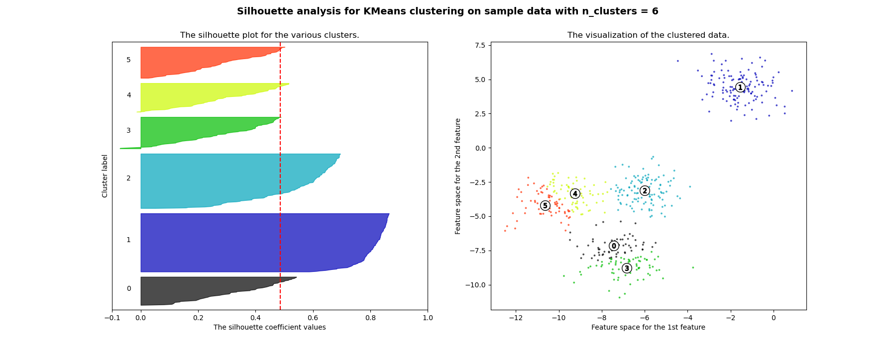
Silhouette Score
Formula:
For each sample, calculate \(s = \frac{b-a}{\max(a,b)}\), where \(a\) is mean distance to samples in same cluster, \(b\) is the mean distance to samples in nearest cluster.
For whole clustering, we average s over all samples.
This scoring prefers compact clusters (like K-means).
Rationale: we want to maximize the difference between \(b\) and \(a\), so that the result is decoupling and cohesion (sounds like object-oriented programming hah?)
Cons: While compact clusters are good, compactness doesn’t allow for complex shapes.
Sample code for choosing evaluation metrics in sklearn
# default scoring for classification is accuracy
scores_default = cross_val_score(SVC(), X, y)

# providing scoring="accuracy" doesn't change the results
explicit_accuracy =  cross_val_score(SVC(), X, y, scoring="accuracy")

# using ROC AUC
roc_auc =  cross_val_score(SVC(), X, digits.target == 9, scoring="roc_auc")

# Implement your own scoring function
def few_support_vectors(est, X, y):
    acc = est.score(X, y)
    frac_sv = len(est.support_) / np.max(est.support_)
    # I just made this up, don't actually use this
    return acc / frac_sv

param_grid = {'C': np.logspace(-3, 2, 6)}
grid = GridSearchCV(SVC(), param_grid=param_grid, cv=10, scoring=few_support_vectors)
Dimensionality Reduction
Linear, Unsupervised Transformation – PCA
PCA rotates the dataset so that the rotated features are statistically uncorrelated. It first finds the direction of maximum variance, and then finds the direction that has maximum variance but at the same time is orthogonal to the first direction (thus making those two rotated features not correlated), so on and so forth.
When to use: PCA is commonly used for linear dimension reduction (select up to first k principal components), visualization of high-dimensional data (draw first v.s. second principal components), regularization and feature extraction (for example, comparing distance in pixel space does not really make sense; maybe using PCA space will perform better)
Whitening: rescale the principal components to have the same scale; Same as using StandardScaler after perfoming PCA.
Why PCA (in general) works
PCA finds uncorrelated components that maximizes the variance explained in the data. However, only when the data follows Gaussian distribution, zero correlation between components implies independence, as the first and second order statistics already captures all the information. This is not true for most of the other distributions.
Therefore, PCA ‘sort of’ makes an implicit assumption that data is drawn from Gaussian, and works the best when representing multivariate normally distributed data.
Important notes
- PCA, compared to histograms or other tools, is used because it can capture the interactions between features.
- Do scaling before performing PCA. Imagine one feature with very large scale. Without scaling, it’s guaranteed to be the first principal component!
- PCA is unsupervised, so it does not use any class information.
- PCA has no guarantee that the top k principal components are the dimensions that contains most information. High variance \(!=\) most information!
- Max number of principal components min(n_samples, n_features).
- Sign of the principal components does not mean anything.
- There’s cancellation effects because of the negative components.
Sample Code
pca_lr = make_pipeline(StandardScaler(), PCA(n_components=2), LogisticRegression(C=1))
pca_lr.fit(X_train, y_train)

pca = PCA(n_components=100, whiten=True, random_state=0).fit(X_train)
X_train_pca = pca.transform(X_train)
X_test_pca = pca.transform(X_test)
Unsupervised Transformation – NMF
NMF stands for non-negative matrix factorization. It is similar to PCA in the sense that it is also a linear, unsupervised transformation. But instead of requiring each componenet to be orthogonal, we want the coefficients to be non-negative in NMF. Therefore, NMF only works to data where each feature is non-negative.
Pros:
- NMF leads to more interpretable components than PCA
- No cancellation effect like PCA
- No sign ambiguity like in PCA
- Can learn over-complete representation (components more than features) by asking for sparsity
- Can be vised as a soft clustering
- Traditional Nonnegative Matrix Factorization (NMF) is a linear and unsupervised algorithm. But there are novice ones that can extract non-linear features (http://ieeexplore.ieee.org/document/7396284/?reload=true)
Cons:
- Only works on non-negative data
- Can be slow on large datasets
- Coefficients not orthogonal
- Components in NMF are not ordered – all play an equal part (also can be a pro)
- Number of components totally change the set of components.
- Non-convex optimization; Randomness involved in initialization
Other matrix factorizations:
- Sparse PCA: components orthogonal & sparse
- ICA: independent components
Non-linear, unsupervised transformation - t-SNE
t-distributed stochastic neighbor embedding (t-SNE) is an algorithm in the category of manifold learning. The high level idea of t-SNE is that it will find a two-dimensional representation of the data such that if they are ‘similar’ in high-dimension, they will be ‘closer’ in the reduced 2D space. To put it in another way, it tries to preserve the neighborhood information.
How t-SNE works: it starts with a random embedding, and iteratively updates points to make close points close.
The usage for t-SNE is now more on data visualization.
Note
- t-SNE does not support transforming new data, so no transform method in sklearn
- Axes do not correspond to anything in the input space, so merely for visualization purpose.
- To tune t-SNE, tune perplexity (low perplxity == only close neighbors) and early_exaggeration parameters, though the effects are usually minor.
Linear, supervised transformation – Linear Discriminant Analysis
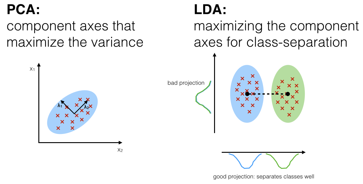
Linear Discriminant Analysis is a “supervised” generative model that computes the directions (“linear discriminants”) that will maximize the separation between multiple classes. LDA assumes data to be drawn from Gaussian distributions (just as PCA, but for each class). It further assumes that features are statistically independent, and identical covariance matrices for every class.
LDA can be used both as a classifier and a dimensionality reduction techinique. The advantage is that it is a supervised model, and there’s no parameters to tune. It is also very fast since it only needs to compute means and invert covariance matrices (if number of features is way less than number of samples).
A variation is Quadratic Discriminant Analaysis, where basically each class will have separate covariance matrices.
Outlier detection
Elliptic Envelope
Assumption:
Data come from a known distribution (for example, Gaussian distribution).
Rationale: Define the “shape” of the data, and can define outlying observations as observations which stand far enough from the fit shape.
Implementation:
- estimate the inlier location and covariance in a robust way (i.e. whithout being influenced by outliers).
- The Mahalanobis distances obtained from this estimate is then used to derive a measure of outlyingness.
Note:
- Only works if Gaussian assumption is reasonable
- Preprocessing with PCA might help
Kernel Density2
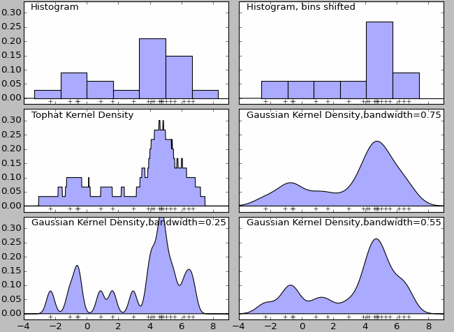
Kernel density estimation is a non-parametric density model. Essentially it is a natural extension of histogram. The density function for histogram is not smooth, and it can be largely affected by the width of the bin. Finally, histogram won’t work with high-dimension data – all these problems can be addressed by kernel density estimation.
Code:
kde = KernelDensity(bandwidth=3)
kde.fit(X)
pred = kde.score_samples(X_test)
One class SVM
One class SVM also uses Gaussian kernel to cover data. It requires the choice of a kernel and a scalar parameter to define a frontier. The RBF kernel is usually chosen as the kernel. The \(\nu\) parameter, also known as the margin of the One-Class SVM (percentage of training mistakes), corresponds to the probability of finding a new, but regular, observation outside the frontier.
Note:
As usual for SVM, do standard scaler before applying OneClassSVM is common practice.
Code:
from sklearn.svm import OneClassSVM
oneclass = OneClassSVM(nu=0.1).fit(X)
pred = oneclass.predict(X_test).astype(np.int)
Isolation Forests
The idea is to build a random tree and we expect that outliers are easier to isolate from the rest, since it is alone. Then we consider the path length for isolating each data point to determine who’s the outlier.
Normalizing path length
\[c(n) = 2H(n-1) - (2(n-1)/n)\]\(s(x,n) = 2^{-\frac{E(h(x))}{c(n)}}\), where \(h\) is the depth of the tree.
s close to 1 meaning it is likely to be outlier.
Building the forest
- Subsample dataset for each tree
- Default sample size of 256 works surprisingly well
- Stop growing tree at depth \(\log_2{n}\) –- so 8 No bootstrapping usually
- The more trees the better (default is 100 trees)
- Need to specify contamination rate (float in 0 to 0.5), default 0.1.
Code:
from sklearn.ensemble import IsolationForest
clf = IsolationForest(max_samples=100, random_state=4, contamination=0.05)
clf.fit(X_train)
y_pred_train = clf.predict(X_train)
Working with imbalanced data
Change threshold
y_pred = lr.predict_proba(X_test)[:, 1] > .85 # change threshold to 0.85
Sanity check question: for the above code, would you expect the precision of predicting positive (class 1) to increase or decrease? How about recall? How about support?
Sampling approaches
Random undersampling
Drop data from the majority class randomly, until balanced.
Pros: very fast training, really good for large datasets
Cons: Loses data
from imblearn.under_sampling import RandomUnderSampler

rus = RandomUnderSampler(replacement = False)
X_train_subsample, y_train_subsample = rus.fit_sample(X_train, y_train)
Use make_pipeline in imblearn:
from imblearn.pipeline import make_pipeline as make_imb_pipeline
undersample_pipe = make_imb_pipeline(RandomUnderSampler(), LogisticRegressionCV())
scores = cross_val_score(undersample_pipe, X_train, y_train, cv=10)
Random oversampling
Repeat data from the minority class randomly, until balanced.
Pros: more data (although many duplication)
Cons: MUCH SLOWER (and sometimes, the accuracy will get lower)
from imblearn.pipeline import make_pipeline as make_imb_pipeline
oversample_pipe = make_imb_pipeline(RandomOverSampler(), LogisticRegressionCV())
scores = cross_val_score(oversample_pipe, X_train, y_train, cv=10)
Class-weights
Instead of repeating samples, we can just re-weight the loss function. It has the same effect as over-sampling (though not random), but not as expensive and time consuming.
from sklearn.linear_model import LogisticRegression
scores = cross_val_score(LogisticRegression(class_weight="balanced"), X_train, y_train, cv=5)
Ensemble resampling
Random resampling for each model, and then ensemble them.
Pros: As cheap as undersampling, but much better results
Cons: Not easy to do right now with sklearn and imblearn
# Code for Easy Ensemble
probs = []
for i in range(n_estimators):
	est = make_pipe(RandomUnderSampler(), DecisionTreeRegressor(random_state=i))
	est.fit(X_train, y_train)
	probs.append(est.predict_probab(X_test, y_test))
pred = np.argmax(np.mean(probs, axis=0), axis=1)
Edited Nearest Neighbors
Remove all samples that are misclassified by KNN from training data (mode) or that have any point from other class as neighbor (all). Can be used to clean up outliers or boundary cases.
from imblearn.under_sampling import EditedNearestNeighbours

# what? it's NearestNeighbours with u and n_neighbors without u
# @.@ Great API design...
enn = EditedNearestNeighbours(n_neighbor=5)
X_train_enn, y_train_enn = enn.fit_sample(X_train, y_train)

enn_mode = EditedNearestNeighbours(kind_sel = "mode", n_neighbor=3)
X_train_enn_mode, y_train = enn_mode.fit_sample(X_train, y_train)
Condensed Nearest Neighbors
Iteratively adds points to the data that are misclassified by KNN. Contrast to Edited Nearest Neighbors,this resampling method focuses on the boundaries.
from imblearn.under_sampling import CondensedNearestNeighbour
# CNN is not convolutional neural net XD
cnn_pipe = make_imb_pipeline(CondensedNearestNeighbour(), LogisticRegressionCV())
scores = cross_val_score(cnn_pipe, X_train, y_train, cv=10)
Synthetic Minority Oversampling Technique (SMOTE)
Add synthetic (artificial) interpolated data to minority class.
Algorithm
- picking random neighbors from k neighbors.
- pick a point on the line between those two uniformly.
- repeat.
Pros: allows adding new interpolated samples, which works well in practice; There are many more advanced variants based on SMOTE.
Cons: leads to very large datasets (as it is doing oversampling), but can be mitigated by combining with undersampled data.
from imblearn.over_sampling import SMOTE
smote_pipe = make_imb_pipeline(SMOTE(), LogisticRegressionCV())
scores = cross_val_score(smote_pipe, X_train, y_train, cv=10)
Clustering and Mixture Model
K-Means algorithm
Algorithm:
- Pick number of clusters k.
- Pick k random points as “cluster center”.
- While cluster centers change:
– Assign each data point to it’s closest cluster center.
- Recompute cluster centers as the mean of the assigned points.
Code:
km = KMeans(n_clusters=5, random_state=42)
km.fit(X)
print(km.cluster_centers_.shape)
# km.labels_ is basically the predict
print(km.labels_shape)
print(km.predict(X).shape)
Note:
- Clusters are Voronoi-diagrams of centers, so always convex in space.
- Cluster boundaries are always in the middle of the centers.
- Cannot model covariance well.
- Cannot ‘cluster’ complicated shape (say two-moons dataset, which I usually refer to as the dataset where two bananas “interleaving” together).
- K-means performance relies on initialization. By default K-means in sklearn does 10 random restarts with different initializations.
- When dataset is large, consider using random, in particular for MiniBatchKMeans.
- k-means can also be used as fetaure extraction, where cluster membership is the new categorical feature and cluster distance is the continuous feature.
Agglomerative clustering
Algorithm:
- Start with all points in their own cluster.
- Greedily merge the two most similar clusters until reaching number of samples required.
Merging criteria:
- Complete link (smallest maximum distance).
- Average linkage (smallest average distance between all pairs in the clusters.
- Single link (smallest minimum distance).
- Ward (smallest increase in with-in cluster variance, which normally leads to more equally sized clusters).
Pros:
- Can restrict to input “topology” given by any graph, for example neighborhood graph.
- Fast with sparse connectivity.
- Hierarchical clustering gives more holistic view, can help with picking the number of clusters.
Cons:
- Some linkage criteria may lead to very imbalanced cluster sized (depending on the scenario, it can be a benefit!).
Code:
from sklearn.cluster import AgglomerativeClustering
for connectivity in (None, knn_graph):
	for linkage in ('ward', 'average', 'complete'):
		clustering = AgglomerativeClustering(linkage=linkage, connectivity=connectivity, n_clusters=10)
		clustering.fit(X)
DBSCAN
Algorithm:
- Sample is “core sample” if more than min_samples is within epsilon (“dense region”).
- Start with a core sample.
- Recursively walk neighbors that are core-samples and add to cluster.
- Also add samples within epsilon that are not core samples (but don’t recurse)
- If can’t reach any more points, pick another core sample, start new cluster.
- Remaining points are labeled outliers.
Pros:
- Can cluster well in complex custer shapes (two-moons would work!)
- Can detect outliers
Cons:
- Needs to adjust parameters (epsilon is hard to pick)
Mixture Models
(Gaussian) Mixture Model is a generative model, where we assume that the data is formed in a generating process.
Assumptions: – Data is mixture of small number of known distributions (in GMM, it’s Gaussian). Each mixture component follows some other distribution (say, multinomial) – Each mixture component distribution can be learned “simply”. – Each point comes from one particular component.
EM algorithm:
- This is a non-convex optimization problem, so gradient descent won’t work well.
- Instead, sometimes local minimum is good enough, and we can get there through Expectation Maximization algorithm (EM)
Code:
from sklearn.mixture import GassuainMixture
gmm = GaussianMixture(n_components=3)
gmm.fit(X)
print(gmm.means_) # If X is of two dimension, returns 3 2D vectors
print(gmm.covariances_) # If X is of two dimension, returns 3 2x2 matrices
gmm.predict_proba(X) # For each data point, what is the probability of it being in each of the three classes?
print(gmm.score(X)) # Compute the per-sample average log-likelihood of the given data X.
print(gmm.score_samples(X)) # Compute the weighted log probabilities for each sample. Returns an array
Note:
- In high dimensions, covariance=”full” might not work.
- Initialization matters. Try restarting with different initializations.
- It allows partial_fit, meaning you can evaluate the probability of a new point under a fitted model.
Bayesian Infinite Mixtures
Note:
- Bayesian treatment adds priors on mixture coefficients and Gaussians, and can unselect components if they do not contribute, so it is possibly more robust.
- Infinite mixtures replace Dirichlet prior over mixture coefficients by Dirichlet process, so it can automatically find number of components based on prior.
- Use variational inference (as opposed to gibbs sampling).
- Needs to specify upper limit of components.
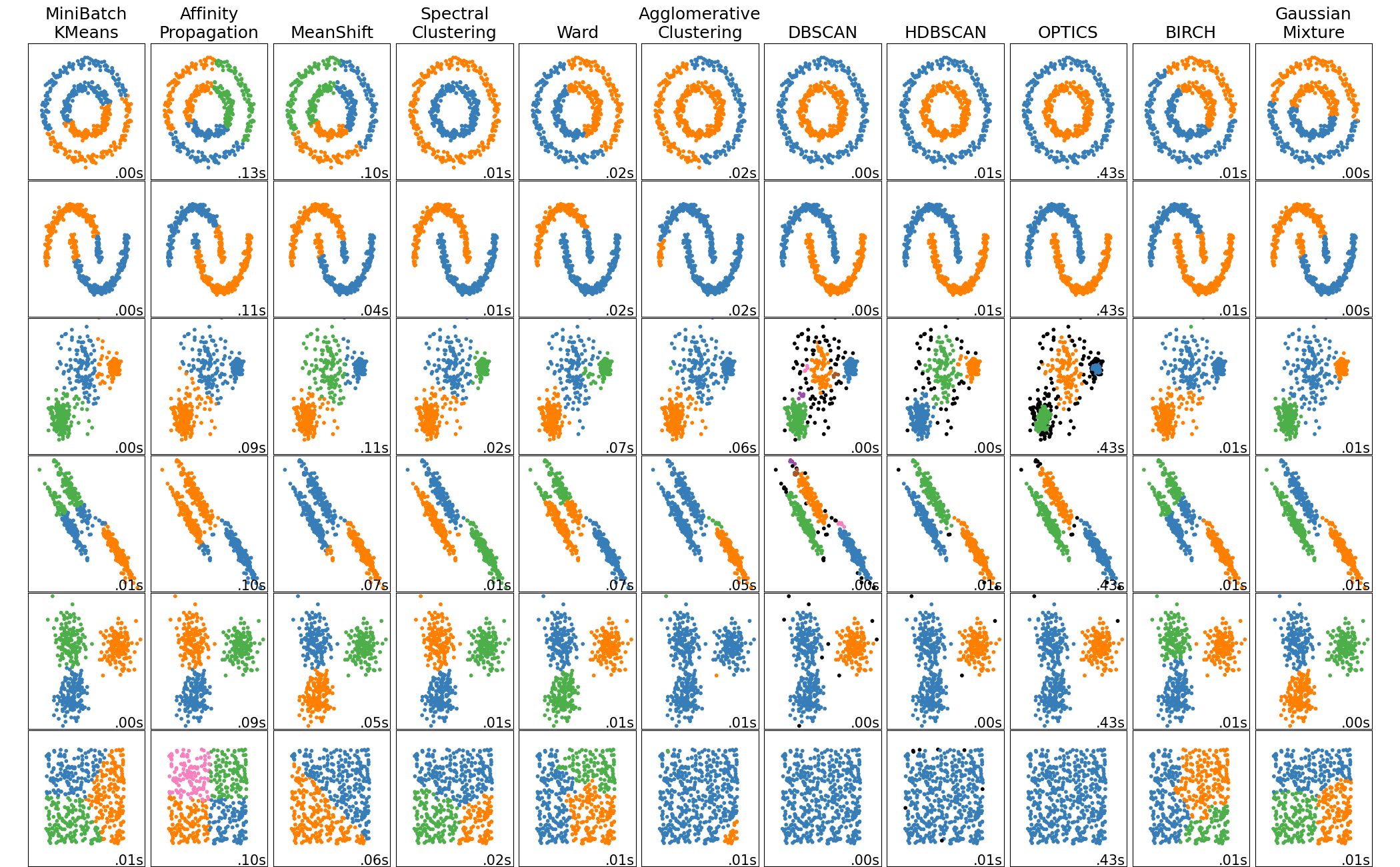
A zoo of clustering algorithm 3
On picking the “correct” number of clusters
Sometimes, the right number of clusters does not even have a deterministic answer. So very likely manual check needs to be involved at the end.
But there are some tools that may be helpful:
Silhouette Plots 4
Cluster Stability
The idea is that the configuration that yields the most consistent result among perturbations is best.
Idea:
- Draw bootstrap samples
- Do clustering
- Store clustering outcome using origial indices
- Compute averaged ARI
Qualitative Evaluation (Fancy name for eyeballing)
Things to look at:
- Low-dimension visualization
- Individual points
- Clustering centers (if available)
GridSearchCV (if doing feature extraction)
km = KMeans(n_init = 1, init = "random")
pipe = make_pipeline(km, LogisticRegression())
param_grid = {'kmeans__n_clusters': [10, 50, 100, 200, 500]}
grid = GridSearchCV(pipe, param_grid, cv=5)
grid.fit(X,y)
n_clusters: For preprocessing, larger is often better; for exploratory analysis: the one that tells you the most about the data is the best.
Natural Language Processing
Generating features from text
The idea of bag of words is to tokenize the text, and then build a vocabulary over all documents, and finally do sparse matrix encoding on each token.
Code:
from sklearn.feature_extraction.text import CountVectorizer
vect = CountVectorizer()
vect.fit(word)
print(vect.get_feature_names())
X = vect.transform(word)
print(vect.inverse_transform(X)[0]) # to see the bag
Tokenization
There are many options:
- Specify token pattern: do you want numbers? single-letter words? punctuations? Specify by regex in CountVectorizer’s token_pattern.
Normalization (preprocessing)
- Correct the spelling
- Stemming: reduce to word stem (by a crude heuristic process that chops off the ends of words in the hope of achieving this goal correctly most of the time, and often includes the removal of derivational affixes)
- Lemmatization: reduce words to stem using curated dictionary and context (properly with the use of a vocabulary and morphological analysis of words, normally aiming to remove inflectional endings only and to return the base or dictionary form of a word, which is known as the lemma)
- Lowercase the words
Restricting the vocabulary (feature selection)
Stop words: exclude some common words using some built-in language-specific / context-specific dictionarys:
vect = CountVectorizer(stop_words='english')
vect.fit(word)
# Use your own stop words
my_stopwords = set(ENGLISH_STOP_WORDS)
my_stopwords.remove("not")
vect3msw = CountVectorizer(stop_words=my_stopwords)
Note: For supervised learning often little effect on large corpuses (on small corpuses and for unsupervised learning it can help)
Max_df: exclude too common word by either setting a percentage or the specific number of occurance threshold
Infrequent words: set min_df with the rationale that words only appear once or twice may not be helpful.
Beyond unigram (Feature engineering)
We can do N-grams: tuples of consecutive words.
cv = CountVectorizer(ngram_range=(1,2)).fit(word)
Note: if you choose really high n-grams, the feature space dimension can explode!
Stop words on bi-gram or 4-gram drastically reduces number of features.
We can do Tf-idf rescaling.
\[tf-idf(t,d) = tf(t,d) \cdot (\log{\frac{1+n_d}{1+df(d,t}} + 1)\]Tf-idf emphasizes rare words, so acting like a soft stop word removal.
It has slightly non-standard smoothings. By default also L2 normalization.
from sklearn.feature_extraction.text import Tfidftransformer
malory_tfidf = make_pipeline(CountVectorizer(), TfidfTransformer()).fit_transform(malory)
We can do character n-grams.
Why?
- Be robust to misspelling
- Language detection
- Learn from names/made-up words
- We think a certain character combination may be a good feature
Analyzer ‘char_wb’ creates character n-grams only from text inside word boundaries. It adds a space before and after each document and can generate larger vocabularies than ‘char’ sometimes. (See here)
cv = CounterVectorizer(analyzer='char_wb').fit(word)
We can include other features.
- Length of text
- Number of out-of-vocabularly words
- Presence / frequency of ALL CAPS
- Punctuation….!? (somewhat captured by char ngrams)
- Sentiment words (good vs bad)
- Domain specific features
Large scale text vectorization – hashing
When doing large scale text vectorization, instead of encoding each token in the vocabulary, we encode the hash value of each token in the vocabulary.
Pro:
- Fast
- Works for streaming data (can do one by one)
- Low memory footprint
- Collisions are not a problem for performance
Con:
- Can’t interpret results
- Hard to debug
Beyond Bag of Words
When doing bag of words, it is hard to capture the semantics of words. Also, synonymous words are not presented, and the representation of documents is very distributed. We are considering other ways to represent a document
Latent Semantic Analysis (LSA)
- Reduce dimensionality of data.
- Can’t use PCA: can’t subtract the mean (sparse data)
- Instead of PCA: Just do SVD, truncate.
- “Semantic” features, dense representation.
- Easy to compute – convex optimization
from sklearn.preprocessing import MaxAbsScaler
# To get rid of some dominating words in a lot of components
X_scaled = MaxAbsScaler().fit_transform(X_train)

from sklearn.decomposition import TruncatedSVD
lsa = TruncatedSVD(n_components=100)
X_lsa = lsa.fit_transform(X_scaled)
Topic Models
We view each document as a mixture of topics. For example, this document can be viewed as a mixture of computer science, applied machine learning and review notes (really bad topic selection…)
We can do NMF for topic models, where we decompose the matrix (document x words) to H and W where H is topic proportions per document and W is topics.
We can also do LDA – Latent Dirichlet Allocation for topic modelling. LDA is a Bayesian graphical generative probabilistic model. The learning is done through probabilistic inference. This is a non-convex optimization and solving it can even be harder than mixture models.
Two solvers:
- Gibbs sampling using MCMC: very accurate but very slow
- Variational inference: faster, less accurate, championed by Prof. David Blei
Rule of thumbs for picking solver:
- Less than 10k documents: use Gibbs sampling
- Medium data: variational inference
- Large data: Stochastic Variational Inference (which allows partial_fit for online learning)
Word embedding
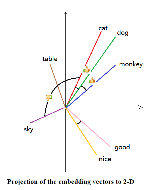
Before we are embedding documents into a continuous, corpus-specific space. Another approach is to embed words in a general space. We want this embedding to preserve some properties: for example: two words that are semantically close should be closer in the mapped vector space.
For example: if we have three words: ape, human and intelligence. If we were using one-hot encoding, we would represent each as [1,0,0], [0,1,0] and [0,0,1], which is sparse and unnecessary (esp when we have A LOT OF WORDS!).
Word embedding may choose to represent them as [0,1], [0.4,0.9] and [1,0]. We have lower dimension, and we kind of preserve the semantics.
As an illustration, see the picture below5:
CBOW
C-BOW stands for continuous bag-of-words. It tries to predict the word given its context. Prediction is done using a one-hidden-layer neural net, where the hidden layer corresponds to the size of the embedding vectors. The prediction is done using softmax. The model is learned using SGD sampling words and contexts from the training data.
Skip-gram
Skip-gram takes the word itself as input and predict the context given the word. You’re “skipping” the current word (and potentially a bit of the context) in your calculation and that’s why it is called skip-gram. The result can be more than one word depending on your skip window. Skip-gram is better for infrequent words than CBOW.
Wait… but why we are doing that?
We don’t really care about the result of CBOW or Skip-gram. Even if we do, the thing that relates to word embedding is that we hope the neural network will learn some useful representation of words in the hidden layer, and that, as a by-product, is what we want here.
Gensim
Gensim has multiple LDA implements and has great tools for analyzing topic models.
texts = [["good", "luck", "with", "your", "final"], ["get", "good", "grade"]]
from gensim import corpora
dictionary = corpora.Dictionary(texts)

corpus = [dictionary.doc2bow(text) for text in texts]

# To convert to sparse matrix
gensim.matutils.corpus2csc(corpus)

# To convert from sparse matrix
sparse_corpus = gensim.matutils. Sparse2Corpus(X.T)

# Tf-idf with gensim
tfidf = gensim.models.TfidfModel(corpus)

# Tokenize the input using only words that appear in the vocabular used in the pre-trained model
vect2_w2v = CountVectorizer(vocabular=w.index2word).fit(text)

# Examples with Gensim
w.most_similar(positive=["Germany","pizza"], negative=["Italy"], topn=3)
There may be stereotype / bias involved here!! (Ethics alert)
We can also do Doc-2-vec: where we add a vector for each paragraph / document, also randomly initialized. (another layer of complexity).
To infer for new paragraph: keep weights fixed, do stochastic gradient descent on the representation D, sampling context examples from this paragraph.
model = gensim.models.doc2vec.Doc2Vec(size=50, min_count=2, iter=55)
model.build_vocab(train_corpus)
model.train(train_corpus, total_examples=model.corpus_count)

# To do encoding using doc2vec:
vectors = [model.infer_vector(train_corpus[doc_id].words) for doc_id in range(len(train_corpus))]
Other things:
GloVe: Global Vectors for Word Representation
Neural Networks
Neural networks is a non-linear model for both classification and regression. It works particularly well when the data set is large. It can basically learn any (continuous) functions. It is a non-convex optimization and is very slow to train (so need GPU resources) There are many variants on this and it is an active research field in machine learning.
General architecture
The general architecture of (vanilla) neural networks looks like this:
Input -> Hidden Layer 1 -> Non-linearity -> Hidden Layer 2 -> Non-linearity -> … -> Hidden Layer n -> (Different) Non-linearity -> Output
Where each layer contains many unit of neuron. For non-linearity, some common selections include: sigmoid, tanh (may get smoother boundaries in small datasets), relu (rectifying linear function, preferred for large network). For the last non-linearity though, we usually use a different function: identity for regression, and soft-max for classification.
Back-propagation
Back-propagation provides a way to compute the update of the weights easily. It combines chain rule and dynamic programming to systematically calculate partial derivatives layer by layer, starting from the last layer, without doing duplicate works.
Note that back-propagation itself does not optmize the weights of a neural network – It is gradient descent or other optimizer that optimizes the weight.
Solvers
The standard solvers include l-bfgs, newton and cg, but if computing gradients over whole dataset is expensive, it is better to use stochastic gradient descent, or minibatch update.
Similarly, constant step size \(\eta\) is not good. A better way is to adaptively learn \(\eta\) for each entry. There’s also adam, which uses a magic number for \(\eta\).
Rule of thumbs for picking solvers:
- Small dataset: off the shelf like l-bfgs
- Big dataset: adam
- Have time & nerve: tune the schedule
Complexity control
- Number of parameters
- Regularization
- Early stopping
- Drop-out
Autodiff
Autodiff is the process to automatically calculate differentiation (usually when you are doing back propagation).
Below is an example: 6
class array(object) :
        """Simple Array object that support autodiff."""
        def __init__(self, value, name=None):
            self.value = value
            if name:
                self.grad = lambda g : {name : g}

        def __add__(self, other):
            assert isinstance(other, int)
            ret = array(self.value + other)
            ret.grad = lambda g : self.grad(g)
            return ret

        def __mul__(self, other):
            assert isinstance(other, array)
            ret = array(self.value * other.value)
            def grad(g):
                x = self.grad(g * other.value)
                x.update(other.grad(g * self.value))
                return x
            ret.grad = grad
            return ret

    # some examples
    a = array(1, 'a')
    b = array(2, 'b')
    c = b * a
    d = c + 1
    print d.value
    print d.grad(1)
    # Results
    # 3
    # {'a': 2, 'b': 1}
When you run d.grad(1), it recursively invokes the grad function of its inputs, backprops the gradient value back, and returns the gradient value of each input. It can be done because gradient calculation is sort of automatically ‘done’ while you perform addition and multiplication: we are keeping track of that computation and building up a graph of how to compute the gradient of it.
Calculate number of parameters in neural network
It’s really nothing fancy. For vanilla neural network, to calculate number of parameters in one layer, it is # of input \(\times\) # of output + # of output (for bias). It will be a bit trickier for convolutional neural network, where you need to take the kernel size into account: width \(\times\) height \(\times\) depth (number of filters we would like to use) \(\times\) (kernel size (including channel!) + 1 (for bias)) (Without parameter sharing).
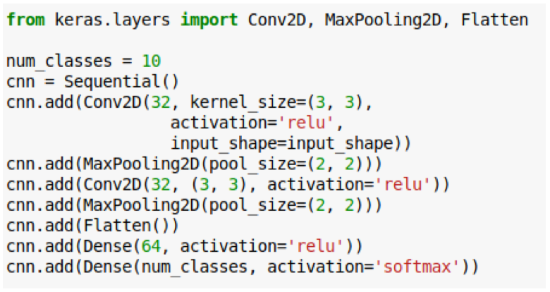
Keras
Keras is an open source neural network library written in Python. It is capable of running on top of Tensorflow or Theano. The API is pretty straightforward (at least the sequencial one). Sequential provides a way to specify feed-forward neural network, one layer after another.
Note
-
For the first layer we need to specify the input shape so the model knows the sizes of all the matrices. The following layers can infer the sizes from the previous layers.
-
The process is:
- Specifying the model (using a list or
.add) model.compile, with optimizer, loss, metrics, validation_split etc. specified.- Do
model.fit, where the training starts - Evaluate on test set by
model.evaluate(X,y,verbose=0), returns loss and accuracy as a tuple.
- Specifying the model (using a list or
Necessary preparation
-
Flatten the data to (num_sample, num_params) (or reshape the data to either (num_samples, width, height, channel) or (num_samples, channel, width, height)), but don’t mess up with the dimension when doing convolutional neural net with images! (meaning when you reshape, you cannot brute force – you should roll/swap the axes and make sure after the reshaping, the image preserves.
-
Standardize so the model will become more stable and is much easier to train when the input is small numbers. Make sure you change to float before the standarization!!! Otherwise you will get all zeros because of the integer division in Python 2… (say this with tears)
-
Do
keras.utils.to_categorical(y_train, num_classes)to do “one-hot” encoding for y. -
Batch size is not a hyperparameters. Instead of gridsearching over it, keep increasing the batch size until you see above 90% GPU utilization.
-
Number of epochs can be tuned by manual tuning, early stopping, or callback.
-
Epochs is fit parameter, not in make_model.
Code
Use callable to wrap the keras and send it to keras classifier:
from keras.wrappers.scikit_learn import KerasClassifier
from sklearn.model_selection import GridSearchCV

def make_model(optimizer="adam", hidden_size=32):
    model = Sequential([
        Dense(hidden_size, input_shape=(784,)),
        Activation('relu'),
        Dense(10),
        Activation('softmax'),
    ])
    model.compile(optimizer=optimizer, loss="categorical_crossentropy", metrics=['accuracy'])
    return model

clf = KerasClassifier(make_model)

param_grid = {'epochs': [1, 5, 10],  # epochs is fit parameter, not in make_model!
              'hidden_size': [32, 64, 256]}

grid = GridSearchCV(clf, param_grid=param_grid, cv=5)
Drop-out regularization
We set some nodes to 0. And not only on the input layer, also the intermediate layer. For each sample, and each iteration we pick different nodes. Randomization avoids overfitting to particular examples.
Rate is often as high as 50%. When predicting, use all weights and down-weight by rate.
When to use drop-out:
- Avoids overfitting
- Allows using much deeper and larger models
- Slows down training somewhat
- Wasn’t able to produce better results on MNIST (I don’t have a GPU) but should be possible
Code
from keras.layers import Dropout

model_dropout = Sequential([
    Dense(1024, input_shape=(784,), activation='relu'),
    Dropout(.5),
    Dense(1024, activation='relu'),
    Dropout(.5),
    Dense(10, activation='softmax'),
])
model_dropout.compile("adam", "categorical_crossentropy", metrics=['accuracy'])
history_dropout = model_dropout.fit(X_train, y_train, batch_size=128,
                            epochs=20, verbose=1, validation_split=.1)
Convolutional Neural Network
High level idea: Convolutional Neural Network extends from vanilla neural net by exploiting the fact that input like images has archiecture: an image can be represented as a 3D volume (width, height, depth/channels) and therefore, instead of flattening them and losing this information, each layer of Convolutional Neural Net transforms an input 3D volume to an output 3D volume with some differentiable function that may or may not have parameters. That’s why it can do really powerful thing with much less parameters.
How many neurons fit in each layer 7
We can compute the spatial size of the output volume as a function of the input volume size (W), the receptive field size of the Conv Layer neurons (F), the stride with which they are applied (S), and the amount of zero padding used (P) on the border. You can convince yourself that the correct formula for calculating how many neurons “fit” is given by (W−F+2P)/S+1(W−F+2P)/S+1.
Parameter Sharing
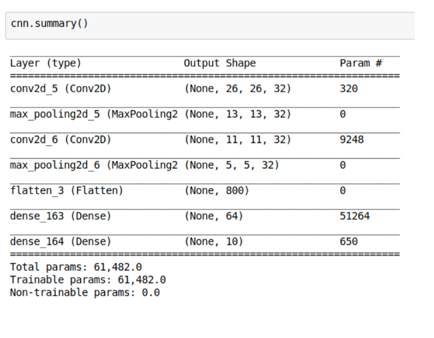
Parameter sharing constrains the neurons in each depth slice (each filter) to use the same weights and bias. Now we only have num of filters \(\times\) (kernel_size (including channel) + 1 (for bias)). Note that the kernel size in the intermediate layer has a depth dimension as # of neurons in the previous layer.
Sanity Check Time: Why the second conv layer has 9248 parameters?
Max pooling
Max pooling is added to progressively reduce the size of the representation to reduce the amount of parameters and computation time. It can also control overfitting.
Sanity check time: A 2x2 max pooling layer gets rid of how many neurons?
Note: Need to remember position of maximum for back-propagation. Again not differentiable so needs to use subgradient descent.
Batch Normalization
Idea: neural networks learn best when the input is zero mean and unit variance. So let’s scale our data – even in the middle
Batch normalization re-normalizes the activations for a layer for each batch during training (as the distribution over activation changes). This happens before applying to activation function (so use BN between the linear and non-linear layers in your network).
Additional scale and shift parameters are learned that are applied after the per-batch normalization.
Use pre-trained networks
Idea: Utilize what people have done with a lot of datasets (“stood on the shoulders of giants”) as feature extraction / as initialization for fine tuning. Usually we will train a last “layer” on top of that, either being logistic regression or a MLP. Also called transfer learning.
Fine tuning: starting with pre-trained net, we back-propagate error through all layers “tune” filters to new data.
Note: This potentially doesn’t work with images from a very different domain, like medical images.
Code:
from keras.applications.vgg16 import preprocess_input
X_pre = preprocess_input(X)
features = model.predict(X_pre)
features_ = features.reshape(200, -1)
Adverserial Samples
Definition: Adverserial samples are samples that were created by an adversary or attacker to fool your model. Usually they learnt the weights in their neural net and cheat by changing the picture slightly. It looks all the same to us, but the neural net will have totally different output.
Given how high-dimensional the input space is, this is not very surprising from a mathematical perspective, but it might be somewhat unexpected.
Time Series
Time Series differs from other data in the sense that it is not iid. (identically and independently distributed). There are equally spaced (like stocks) and non equally spaced (like earthquake data) time series.
Key point: the train/test split and validation set split is different as usual. We must make sure the training data set is in the past and we use those to predict future!
Tasks
- 1D forecasting: one thing, use past predict future
- ND forecasting: multiple things, use past predict future (predict one or more)
- Feature-based forecasting
- Time series classification
Parse date & Time Series Index
The code will combine multiple columns into a single date (so concatenate years, months and days to a date. Furthermore, it treats the newly created column as the index – now pandas will be able to do stuff because this data frame is a time series data frame!
data = pd.read_csv(url, parse_dates=[[0,1,2]], index_col="year_month_day")
Backfil and forward fill
Imputation by looking back or forward
maunaloa.fillna(method="ffill", inplace=True)
Resampling
resampled_co2 = manualoa.co2.resample("MS") # MS is month start frequency
resampled_co2.mean().head() # resampling is lazy -- only until when you use it, it will actually extract out the data
Detrending (look at differencing)
data.diff().plot()
Autocorrelation (correlation between two data point)
data.autocorr(lag=12)
Autoregressive linear model
Model: \(x_{t+k} = c_0x_t + c_1x_{t+1} + \cdots + c_{k-1}x_t\)
from statsmodels.tsa import ar_model
ar = ar_model.AR(ppm[:500])
res = ar.fit(maxlag=12)
res.params
res.predict(ppm.index[500], ppm.index[-1])
Note:
- Change max lag will change the fitting a lot!
ARIMA
from statsmodels import tsa

arima_model = tsa.arima_model.ARIMA(ppm[:500], order=(12, 1, 0))
res = arima_model.fit()
arima_pred = res.predict(ppm.index[500], ppm.index[-1], typ="levels")
With scikit-learn: fit linear/quadratic linear regression
X_train, X_test = X.iloc[:500, :], X.iloc[500:, :]
from sklearn.linear_model import LinearRegression
lr = LinearRegression().fit(X_train, train)
lr_pred = lr.predict(X_test)

from sklearn.preprocessing import PolynomialFeatures
lr_poly = make_pipeline(PolynomialFeatures(include_bias=False), LinearRegression())
lr_poly.fit(X_train, train)
One way to do things is to use a linear model with poly-2 features to learn the trend, and then detrend, and do AR model on residuals.
Side note: pandas group-by function
Can be pretty handy!
week = energy.Appliances.groupby([energy.index.hour, energy.index.dayofweek]).mean()
-
Source: http://sebastianraschka.com/Articles/2014_python_lda.html#principal-component-analysis-vs-linear-discriminant-analysis ↩
-
Source: http://www.dataivy.cn/blog/%E6%A0%B8%E5%AF%86%E5%BA%A6%E4%BC%B0%E8%AE%A1kernel-density-estimation_kde/ ↩
-
Source: http://scikit-learn.org/dev/auto_examples/cluster/plot_cluster_comparison.html ↩
-
Source: http://scikit-learn.org/stable/auto_examples/cluster/plot_kmeans_silhouette_analysis.html ↩
-
Source: https://www.zhihu.com/question/32275069 ↩
-
Source: http://mxnet.io/architecture/program_model.html ↩
-
Source: http://cs231n.github.io/neural-networks-1/ ↩